cell
定义空cell
定义一个2✖️3的元胞结构数组
>> x=cell(2,3)

x =

  2×3 cell 数组

    {0×0 double}    {0×0 double}    {0×0 double}
    {0×0 double}    {0×0 double}    {0×0 double}
cell读取时{}()的区别
- ()读取得到的是元包结构,即cell数组
- {}读取得到的是数据本身的内容,例如字符串
% 这个例子
>> title={{'pitch-RAO'} {'T'}    {'heave-波能俘获效率'} }

title =

  1×3 cell 数组

    {1×1 cell}    {1×1 cell}    {1×1 cell}

>> title(1)

ans =

  1×1 cell 数组

    {1×1 cell}

>> title{1}

ans =

  1×1 cell 数组

    {'pitch-RAO'}

>> title(1)(1)
错误:  无效的数组索引。

>> title(1){1}
错误:  无效的数组索引。

>> title{1}{1}

ans =

    'pitch-RAO'

>> title{1}(1)

ans =

  1×1 cell 数组

    {'pitch-RAO'}
坐标轴科学记数法表示与轴范围的影响
xlim([xmin xmax]) x轴显示范围ylim([ymin ymax]) y轴显示范围xticklabel xtick x坐标轴标签yticklabel ytick x坐标轴标签
介绍
这一行的命令,意思是读取当前坐标轴的刻度值,然后转换为文本进行标记
set(gca,'xticklabel',get(gca,'xtick'),'yticklabel',get(gca,'ytick'));
如果,后续命令需要修改x、y轴的显示大小,如将x轴从[5,20]调整为[0,20],那么需要在设置区间后再改变坐标轴label,通过以下代码展示。
因此如果之后需要调整坐标轴内容,那么一定要注意代码书写顺序。
示例代码
clc
clear
close all
x=[5:20];
y=x.^2;
figure()
% 图1:先将标签修改为文本,然后修改区间显示,文本标签重新调整位置,已经不是真实值
subplot(1,2,1)
plot(x,y,'-*',LineWidth=2)
set(gca,'xticklabel',get(gca,'xtick'),'yticklabel',get(gca,'ytick'));
xlim([0 30]);
title('图1')

% 图2:先调整区间,然后将区间转化为文本,显示正常
subplot(1,2,2)
plot(x,y,'-*',LineWidth=2)
xlim([0 30]);
set(gca,'xticklabel',get(gca,'xtick'),'yticklabel',get(gca,'ytick'));
title('图2')
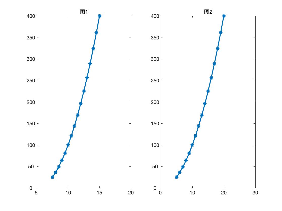
补充命令
关于xlim、ylim的使用,Matlab官网也有文档说明。
xlim
% 获得当前x轴的范围,如[5 20]
xlim([0 20])
% 设定x轴范围为[0 20]

xlim([0 inf])
% 设定x轴范围为从0开始到默认最大;-inf即为默认最小
Unique
数组中的唯一值 - MATLAB unique - MathWorks 中国 https://ww2.mathworks.cn/help/matlab/ref/double.unique.html
语法
C = unique(A)
C = unique(A,setOrder)
C = unique(A,occurrence)
C = unique(A,___,'rows')
C = unique(A,'rows',___)
[C,ia,ic] = unique(___)
[C,ia,ic] = unique(A,'legacy')
[C,ia,ic] = unique(A,'rows','legacy')
[C,ia,ic] = unique(A,occurrence,'legacy')
[C,ia,ic] = unique(A,'rows',occurrence,'legacy')
说明
C = unique(A) 返回与 A 中相同的数据,但是不包含重复项。C 已排序。
- 如果 A 是表或时间表,则 unique 按排序顺序返回 A 中的唯一行。对于时间表,当确定行是否唯一时,unique 会考虑行时间和行值,并按行时间对输出时间表 C 排序。
- 如果 A 是分类数组,则排序顺序由类别的顺序确定。
C = unique(A,setOrder) 以特定顺序返回 A 的唯一值。setOrder 可以是 ‘sorted’(默认值)或 ‘stable’。
C = unique(A,occurrence) 指定遇到重复值时应返回哪个索引。occurrence 可以是 ‘first’(默认值)或 ’last’。
C = unique(A,___,'rows')和 C = unique(A,'rows',___)将 A 中的每一行视为单个实体,并按排序顺序返回 A 中的唯一行。必须指定 A,而 setOrder 和 occurrence 是可选的。‘rows’ 选项不支持元胞数组。
[C,ia,ic] = unique(___) 还可使用上述任何语法返回索引向量 ia 和 ic。
- 如果 A 是向量,则
C = A(ia)且A = C(ic)。 - 如果 A 是矩阵或数组,则
C = A(ia)且A(:) = C(ic)。 - 如果指定了 ‘rows’ 选项,则
C = A(ia,:)且A = C(ic,:)。 - 如果 A 是表或时间表,则
C = A(ia,:)且A = C(ic,:)。
Matlab求取曲线平均值
https://ww2.mathworks.cn/matlabcentral/answers/290707-average-multiple-curves-matlab
x1 = sort(rand(1, 10));                                 % Create Data
y1 = rand(size(x1));                                    % Create Data
x2 = sort(rand(1, 15));                                 % Create Data
y2 = rand(size(x2));                                    % Create Data

xi = linspace(0, 1, 50);                                % Create Vector Of Common X-Values

y1i = interp1(x1(:), y1(:), xi(:), 'linear', 'extrap'); % Interploate Or Extrapolate To New ‘x’ Values
y2i = interp1(x2(:), y2(:), xi(:), 'linear', 'extrap'); % Interploate Or Extrapolate To New ‘x’ Values

y_mean = mean([y1i y2i], 2);                            % Mean Of Y Values

figure(1)
plot(x1, y1, '-b')
hold on
plot(x2, y2, '-g')
plot(xi, y_mean, '-r', 'LineWidth',2)
hold off
grid
legend('Data 1', 'Data 2', 'Data Mean', 'Location','N')
% ---------------------------------------------------------------------------- %
% DESCRIPTION                                                                  %
% -----------                                                                  %
% Returns an average curve of multiple curves by linear interpolation. The     %
% returned average curve also has unique and sorted abscissae.                 %
% ---------------------------------------------------------------------------- %
% INPUT                                                                        %
% -----                                                                        %
% abscissae:                                                                   %
% If this argument is a scalar, it specifies the number of abscissae on which  %
% the average curve is evaluated, automatically ranging from the global        %
% minimum to the global maximum abscissa considering all curves. If this       %
% argument is a vector, the average curve is evaluated in the abscissae        %
% specified by it.                                                             %
%                                                                              %
% curves:                                                                      %
% A cell array of length n containing the data of each curve, where n is the   %
% number of curves. The data of each curve is defined by a two-column matrix,  %
% where the first column corresponds to the abscissae and the second column    %
% corresponds to the ordinates. Each curve may have a different number of      %
% points.                                                                      %
% ---------------------------------------------------------------------------- %
% OUTPUT                                                                       %
% ------                                                                       %
% curve:                                                                       %
% The abscissae and ordinates of the average curve in a two-column matrix.     %
% ---------------------------------------------------------------------------- %

function curve = avgcurve(abscissae, curves)

% determine abscissae
if isscalar(abscissae)
    xmin = +Inf;
    xmax = -Inf;
    for i = 1 : length(curves)
        imin = min(curves{i}(:,1));
        imax = max(curves{i}(:,1));
        if imin < xmin, xmin = imin; end
        if imax > xmax, xmax = imax; end
    end
    x = linspace(xmin, xmax, abscissae)';
else
    x = abscissae(:);
end

% compute ordinates
y = zeros(size(x));
k = zeros(size(x));
for i = 1 : length(curves)
    [xi, ii] = unique(curves{i}(:,1), "first");
    yi = curves{i}(ii,2);
    interp = interp1(xi, yi, x, "linear");
    k = k + ~isnan(interp);
    interp(isnan(interp)) = 0;
    y = y + interp;
end
y = y ./ k;

% done
curve = [x y];